
When the BLS models payroll expansion they don’t actually count payroll expansion. In the 1960’s, economic accounting shifted to mostly stochastic processes which changed the way mainstream economic statistics were calculated and kept. We all know, particularly recently, about how these data series are constantly revised, and often by more than minor adjustments, but that in some ways obscures the reality of what is taking place in them to begin with. There seems to be an unearned reputation for precision that goes way, way beyond actually understanding what monthly variability actually means.
The Establishment Survey in particular has been the one notable account supporting the idea of a gathering recovery. That should be enough since employment levels are typically associated with actual and sustained expansions, yet nothing else has behaved in a manner that would corroborate the BLS’ version of what is going on. Even the unemployment rate itself, derived from the related Household Survey, has been marginally improving more so by the relatively declining labor participation than actual modeled employment gains. This is already not the typical business cycle adherence to predicted correlations.
That has left the BLS at odds with spending and productivity, but most people are not aware of just how subjective all of this statistical “science” can be. The Establishment Survey is taken as the definitive description of economic status while the rest is left usually as noise despite the aberrations that abound there. The gathering slump in 2015 so far, however, has made this dichotomy harder to simply dismiss. Further, large downward revisions just in the past few weeks of retail sales and related durable goods have cast further doubt about the “best payroll expansion in decades” as something real and not just subjective number jiggering.
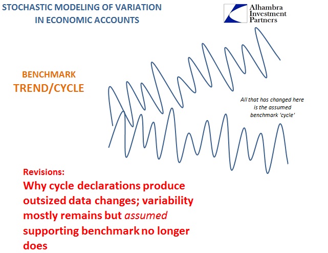
Those consumer spending revisions related to a benchmark re-assessment from a 2012 Census retooling. Essentially, the Census Bureau was too aggressive in its projected path for retail sales (and thus durable goods), which gives away the subjectivity here. Again, the month-to-month figures released, which are taken as actual economic levels, are simply just statistical measures of monthly variation chained together in a harmonized series, all controlled at the start by an assumed level of trend and cycle.
In 1967, in a paper posted on the Census Bureau’s website, authors Julius Shiskin, Allan Young and John Musgrave decompose “seasonal” adjustments by parts in describing the relatively new seasonal format of AutoRegressive Integrated Moving Average templates (ARIMA, then X-11):
There are various and sundry methods for seasonally adjusting economic time series, all of which are based on the premise that seasonal fluctuations can be measured in an original series (O) and separated from the trend, cyclical, trading-day, and irregular functions. The seasonal component (S) is defined as the intrayear pattern of variation which is repeated constantly or in an evolving fashion from year to year. The trend-cycle component (C) includes the long-term trend and business cycle. The trading-day component (TD) consists of variations which are attributed to the composition of the calendar. The irregular component (I) is composed of residual variation, such as the sudden impact of some political events, the effect of strikes, unseasonable weather conditions, reporting and sampling errors, etc. The seasonally adjusted series (CI) consists of the trend-cycle and irregular components.
What “economists” (really statisticians rather than actual experts on economic behavior) found was that in examining variation even in “low frequency components” that trend and cycle were the most important determinant factors. That makes intuitive sense because if the economy is in recession then that downward force will set aside or overwhelm any other forms of variation; the same has been true in recovery and growth. The problem for econometrics and putting together economic accounts is that these various government agencies can only “see” recession in the rearview, and even then only as it has occurred according to past results.
In 1979, Nobel Laureate Clive Granger pointed out:
It can certainly be stated that, when considering the level of an economic variable, the low frequency components, often incorrectly labeled ‘trend-cycle components,’ are usually both statistically and economically important. They are statistically important, because they contribute the major part of the total variance, as the typical spectral results and the usefulness of integrated (ARIMA) models indicates. The economic importance arises from the difficulty found in predicting at least the turning points in the low-frequency components and the continual attempts by central governments to control this component, at least for GNP, employment, price, and similar series.
That makes any analysis considering both trend and cycle highly important, “the major part of total variance”, to modeling economic accounts under the “seasonal” format. What is implied is that trend/cycle is almost binary in its setting.
We think these agencies are delivering the economic picture based on hard data, but in reality there is tremendous guesswork involved. That usually wasn’t much of a problem because the economy had always either been in recession or growth. Prior to the 1990’s, the shape of the economic trajectory was almost exclusively a “V”, which is why Milton Friedman delivered his “plucking model” format for shaping not just understanding but even quantitative monetary policy interests.
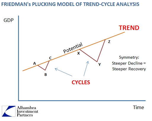
For both high frequency and low frequency data points, estimations of both trend and cycle would form the main relevance to setting benchmarks which are used to chain together those statistical estimates of variation. When the economy is in either recession or growth, there isn’t much controversy about doing so – only in the shift from one to the other and back again, which is what Granger was describing.

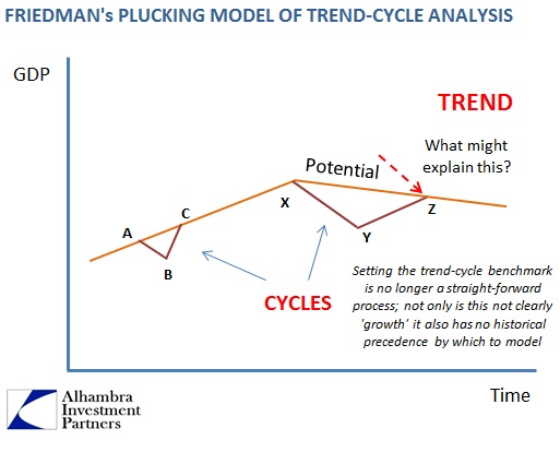
We don’t have much information about how the Census Bureau or the BLS sets its trend-cycle components and estimates, but the revisions of late have suggested what I have suspected for years; namely that they have been overaggressive in their benchmarks, and thus overstating actual economic progress. The reason for that is actually quite simple, in that Friedman’s plucking model itself has been disproved for at least this “cycle”, if not stretching back to the turn of the century. Thus, we have “discovered” a new kind of trend/cycle setting which is somewhat like a growth period but at the same time very much unrelentingly recessionary too.
If trend/cycle is the great determinant of economic account variability, and we have very little actual idea what trend or cycle is dominant right now, then all bets are off; in many ways, these statistics are flying blind.
This has been particularly acute after the 2012 slowdown, and yet the BLS has taken its payroll estimates into overdrive without seeing a commensurate surge in spending or even incomes! I have inferred that they are using jobless claims as a proximate indicator for increasing trend/cycle, but it might be just plain guesswork on their part or even bias over QE3 and QE4 (if you think QE works and your job is to set benchmark growth for coming variations, then might you not over-estimate that benchmark based on nothing more than that mistaken monetary belief?).
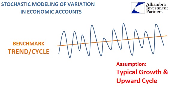
The difference, then, between a more consistent track of payroll “expansion” and the rest of the much more dour economic accounts is left to just faith and guessing. There is no historical basis for this nor is there any way to objectively measure something that hasn’t happened since the 1930’s (the similarities between the current depression-like behavior and the Great Depression should actually be considered here in setting trend-cycle estimates but clearly are being fully set aside). Instead, it appears that statisticians working in these economic accounts are just assuming a typical cycle, which leaves a dramatic potential difference between what they think has happened and what really may be underlying.
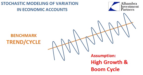
The recent benchmark revisions as well as related statistical oddities (like productivity) increases the odds that the BLS has been using far too optimistic trend-cycle components without much aside from unanchored conjecture in doing so. It may be just shy of five full years now since the Great Recession was declared ended but the current run of economic advance has been nothing like any of the prior periods. So the benchmark setting of the “typical” +5 years from a recession trough doesn’t really apply; economic growth in the past (pre-1990’s) may have shifted into ultra-high growth with very low jobless claims but there is a mountain of evidence and observation now that opposes such a setting for our current, clearly inferior circumstances.
Most of all is the current and gathering economic “slump.” It is highly inconsistent with such robust and sustained jobs expansion, meaning that more than anything else this chronic over-estimation really stands out. The longer this deviation is maintained, the greater the likelihood that the latest “payroll” variation this week will be revised significantly lower – and no one will care on Friday.
The dominant theory on stochastic assembly for economic accounts demands conformity with historical patterns. With that basis obliterated, and with it all forms subscribing to the plucking assumptions, there is an all-too-real danger of greatly over-configuring the positive trend-cycle bias especially the further we get from the last declared cycle. In short, there is a far greater likelihood than is contemplated that payrolls are nothing like the “greatest jobs expansion in decades”, and that eventually it will be recognized as such though far too late to do much about it.
It isn’t just dangerous to follow the statistics blindly and narrowly, it comes down to fooling convention into not taking corrective measures when they might have had some chance to succeed. By offering cover to QE, the economy suffers for all that is assumed QE may have worked, most especially through the payroll reports that are increasingly isolated and questioned. Maybe that is somehow fitting, if tragic, since the FOMC is using the payroll report exclusively to justify ending ZIRP, while at the same time the BLS is using past QE bias to possibly set its trend/cycle that is now being used to judge the success of QE. So much of monetary theory is circular logic, why not one more facet?
Stay In Touch